Traditional neural networks process data in fixed sequences, treating each input independently. This approach struggles with tasks requiring temporal awareness – like language translation or speech recognition. Here’s where recurrent neural networks (RNNs) revolutionise the game.
Unlike their static counterparts, RNNs utilise feedback loops to retain context from previous inputs. Each processing step feeds outputs back into the system, creating an evolving memory bank. This architecture mirrors human cognition, where understanding builds upon prior knowledge.
The real power lies in handling sequential information. Whether analysing stock market trends or composing music, RNNs assess patterns across time steps. Their ability to reference historical data makes them indispensable for predicting next elements in a series.
Modern applications range from voice assistants to medical diagnostics. These systems excel precisely because they don’t “forget” crucial context between processing stages. By maintaining dynamic internal states, RNNs achieve nuanced interpretations that traditional models miss.
Introduction to Recurrent Neural Networks
Machine learning models often struggle with tasks requiring temporal awareness. Unlike static architectures, recurrent neural networks (RNNs) tackle this challenge through built-in memory systems. These systems retain contextual clues across data sequences, enabling predictions based on historical patterns.
What Sets RNNs Apart?
Three core features define these architectures:
- Persistent context: Internal states update dynamically, referencing prior inputs during current analyses
- Sequence mastery: Excel at interpreting ordered information like text or time-series metrics
- Adaptive processing: Adjust interpretations as new data flows through the system
The Role of Memory in Sequential Data
Traditional neural networks treat each input independently. RNNs revolutionise this approach by maintaining evolving memory banks. Stock price predictions illustrate this advantage – yesterday’s trends directly influence today’s forecasts.
Order sensitivity proves critical. Language translation systems, for instance, rely on sentence structure awareness. A misplaced word can alter meaning entirely. RNNs’ ability to track positional relationships makes them indispensable for such applications.
These architectures outperform conventional models in scenarios demanding temporal pattern recognition. Their memory mechanisms capture dependencies between distant data points, something feedforward systems often miss.
Understanding How Does a Recurrent Neural Network Work
Sequential data processing demands architectures that evolve with each new piece of information. This is where systems with cyclical connections shine, leveraging temporal relationships traditional models overlook.
Step-by-Step Process
At every interval, these systems analyse inputs while referencing historical context. A hidden layer maintains an evolving memory bank, updated through mathematical operations combining current data with prior states.
The mechanism follows three principles:
- State persistence: Hidden layers retain processed information using activation functions
- Weight sharing: Identical parameters apply across all processing intervals
- Recursive updates: Current outputs influence subsequent calculations
Consider language prediction: each word’s interpretation depends on preceding terms. The hidden state adjusts dynamically, much like human comprehension builds cumulatively. This approach enables consistent handling of variable-length sequences, from weather patterns to recurrent neural networks in financial forecasting.
Through this looping architecture, systems develop contextual awareness unmatched by static models. Memory isn’t just stored – it’s actively reshaped with each new data point, creating adaptive intelligence for time-sensitive tasks.
Architectural Components of RNNs
The blueprint of these systems hinges on two critical elements that manage sequential dependencies. Specialised processing units collaborate with temporal expansion techniques to handle evolving data streams.
Recurrent Units and Hidden States
Recurrent units act as the system’s memory cells. Each unit maintains a hidden state – a dynamic repository storing historical context. This state updates at every interval, blending fresh inputs with prior knowledge using activation functions.
Parameter sharing ensures consistent processing rules across all time steps. Unlike traditional layers in static models, these units operate cyclically. Their design allows handling phrases in text or fluctuations in sensor readings with equal finesse.
Unfolding RNNs Over Time
Visualising cyclical architectures becomes clearer through temporal unrolling. This technique transforms the compact recurrent structure into an expanded chain of interconnected layers. Each layer represents a specific moment in the sequence.
The unrolled version reveals:
- Information flow between consecutive steps
- Weight replication across temporal layers
- Backpropagation pathways for error correction
This feedforward-like representation enables gradient calculations spanning multiple intervals. Financial analysts might use such expanded models to track quarterly trends, while linguists could map sentence dependencies across paragraphs.
Mathematical Foundations and Key Formulas
Equations drive every prediction in temporal data processing systems. These computations blend historical context with fresh inputs through carefully designed transformations. Let’s examine the arithmetic that powers sequential pattern recognition.
Hidden State and Output Calculations
Core computations follow a structured pattern across intervals. The table below breaks down essential operations:
| Formula Name | Equation | Parameters | Purpose |
|---|---|---|---|
| State Update | ht = tanh(Whhht-1 + Wxhxt) | Whh, Wxh (weights) | Combines previous memory with new data |
| Output Generation | yt = Whyht | Why (output weights) | Transforms hidden state into predictions |
| Full System | Y = f(X, h, W, U, V, B, C) | B (bias), C (output bias) | Defines complete input-output function |
Weight matrices (W) act as transformation filters. They determine how strongly previous states influence current calculations. At each time step, these parameters adjust through learning processes to capture temporal relationships.
The hyperbolic tangent (tanh) serves as the primary activation function here. It squashes values between -1 and 1, preventing numerical explosions during repeated computations. This non-linear behaviour helps models recognise complex patterns in sequences.
Output calculations use simpler linear combinations. The final layer applies task-specific functions – softmax for classification or linear scaling for regression. This layered approach enables single architectures to handle diverse sequential challenges.
Backpropagation Through Time (BPTT)
Training sequential models demands algorithms that account for temporal relationships. Backpropagation Through Time (BPTT) tackles this by unrolling networks across intervals, enabling gradient calculations through historical steps. Unlike standard backpropagation, this method preserves dependencies between distant data points.
Gradient Propagation in Sequences
BPTT calculates errors by reversing the network’s temporal expansion. Each time step contributes to the final loss, creating nested chains of mathematical derivatives. These computations reveal how slight weight adjustments impact outputs across multiple intervals.
Three critical challenges emerge:
- Exponential growth in computational complexity with longer sequences
- Risk of vanishing/exploding gradients during backward passes
- Memory constraints from storing intermediate states
Engineers often use truncated BPTT to balance accuracy and efficiency. This technique processes sequences in chunks rather than full histories. For weather forecasting systems, this approach maintains training viability while capturing weekly patterns.
The algorithm’s true power lies in its adaptability. Financial institutions employ BPTT variants to model stock behaviours, where learning multi-year dependencies proves crucial. Such applications underscore its role in modern temporal analysis frameworks.
Types and Variations of Recurrent Neural Networks
Modern machine learning offers multiple solutions for handling sequential data. Four architectures dominate this space, each addressing unique challenges in temporal pattern recognition.
Core Architectures Compared
Vanilla RNNs form the simplest framework. These single-layer systems share weights across intervals, making them efficient for short-term dependencies. However, they struggle with prolonged sequences due to vanishing gradients.
LSTMs revolutionised long-term memory retention. Their gated architecture features:
- Input gates regulating new information flow
- Forget gates pruning irrelevant historical data
- Output gates controlling prediction content
GRUs streamline this approach. By merging input/forget gates into update mechanisms, they reduce computational demands while maintaining effectiveness. Reset gates further optimise information filtering.
Bidirectional Processing
Some scenarios demand forward and backward sequence analysis. Bidirectional systems process data in both directions simultaneously. This proves invaluable for language translation, where word meaning depends on entire sentence context.
| Type | Key Features | Best Use Cases |
|---|---|---|
| Vanilla RNN | Simple architecture, low complexity | Short text prediction |
| LSTM | Three-gate memory control | Speech recognition |
| GRU | Two-gate efficiency | Real-time analytics |
| Bidirectional | Dual-direction processing | Machine translation |
Choosing the right architecture depends on sequence length and resource constraints. Financial forecasting might favour GRUs for speed, while medical diagnostics could require LSTMs’ precision.
Comparing RNNs with Feedforward Neural Networks
Effective machine learning requires matching architecture to task requirements. Feedforward neural networks operate through rigid, one-way data pipelines – ideal for static tasks like image recognition. These systems process inputs independently, discarding context after each analysis cycle.
This design falters with sequential information. Without memory mechanisms, feedforward architectures struggle to link events across time steps. Stock market predictions or language translation demand awareness of prior data points – a gap recurrent systems fill through cyclical processing.
RNNs’ feedback loops enable dynamic context retention. Hidden states evolve with each input, allowing interpretations to build cumulatively. Such architectures excel in scenarios where outputs depend on historical patterns, like voice assistants interpreting speech rhythms.
Key distinctions:
- Data handling: Feedforward models isolate inputs; RNNs track sequences
- Resource use: Static networks train faster; recurrent systems require temporal optimisation
- Applications: Use feedforward for image classification, RNNs for time-series forecasting
Choosing between these architectures hinges on whether tasks demand memory or prioritise isolated data processing. Each approach serves distinct roles in modern AI ecosystems.
FAQ
What sets RNNs apart from other neural networks?
Unlike feedforward architectures, recurrent neural networks process sequential data by retaining memory of previous inputs. This allows them to handle time series, text, or speech where context and order matter. Hidden states act as a dynamic memory bank, updating at each time step.
How do recurrent units manage long-term dependencies?
Standard RNNs struggle with vanishing gradients over extended sequences. Advanced variants like LSTM (Long Short-Term Memory) and GRU (Gated Recurrent Units) use specialised gates to regulate information flow. These gates decide what to store, update, or discard, mitigating gradient issues.
Why is backpropagation through time used in training?
Backpropagation through time (BPTT) unrolls the network across multiple time steps, enabling gradient calculation for sequential data. This approach adjusts weights based on errors propagated backward, though it faces challenges like exploding gradients in deep architectures.
What are common applications of gated recurrent units?
GRUs excel in machine translation, speech recognition, and time-series forecasting. Their simplified gate structure – reset and update gates – balances computational efficiency with performance, making them popular in real-time systems like Google Translate or Alexa’s voice processing.
How does bidirectional architecture enhance RNN performance?
Bidirectional RNNs process data in both forward and reverse directions. This dual perspective captures context from past and future states simultaneously, improving tasks like sentiment analysis or protein structure prediction where surrounding elements influence outcomes.
What distinguishes LSTMs from vanilla RNNs?
LSTMs introduce input, output, and forget gates alongside a cell state. This design allows precise control over long-term memory retention, outperforming vanilla RNNs in tasks requiring context over extended sequences, such as paragraph generation or video frame analysis.
Why might deep learning models combine RNNs with other layers?
Hybrid architectures, like using convolutional layers with RNNs, leverage spatial feature extraction alongside temporal modelling. For instance, video captioning systems might use CNNs for frame analysis and RNNs to generate descriptive text sequences.


